Programming with Escher
This notebook is a collection of preliminary notes about a "code camp" (or a series of lectures) aimed at young students inspired by the fascinating Functional Geometry paper of Peter Henderson.
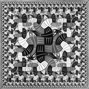
In such work the Square Limit woodcut by Maurits Cornelis Escher is reconstructed from a set of primitive graphical objects suitably composed by means of a functional language.
Here the approach will be somehow different: first of all because our recipients will be students new to computer science (instead of fellow researchers), but also because besides recalling the fundamental concepts of abstraction levels (and barriers), primitives and composition, present in the original paper, we will here also take the opportunity to introduce some (albeit to some extent elementary) considerations on algebra and geometry, programming and recursion (and perhaps discuss some implementation details).
This work is to be considered very preliminary, it is not yet structured in a series of lectures, nor it is worked out the level at which every topic is to be presented, according to the age (or previous knowledge) of the students. The language and detail level used here is intended for instructors and teachers, and the various topics will be listed as mere hints, not yet as a viable and ready to use syllabus.
As a last remark, before actually beginning with the notes, the code of this notebook is very loosely derived from previous "implementations" of Functional Geometry such as Shashi Gowda's Julia version and Micah Hahn's Hasjell version (containing the Bézier curve description of the Escher fish used here). I decided to rewrote such code in a Jupyter notebook written in Python 3, a simple and widespread language, to make it easier for instructors to adopt it.
The source notebook is available on GitHub (under GPL v3), feel free to use issues to point out errors, or to fork it to suggest edits.
Square Limit and tiles
Looking at the original artwork it is evident that it is obtained by the repetition of a basic element (a fish) that is suitably oriented, scaled, and colored.
This suggest to start our journey from a tile (a set of lines enclosed in the unit square), that is a drawing building block, that we will manipulate to obtain more complex drawings.
Note that, if one wants to follow an "unplugged" approach, tiles can be actually printed as objects so that students will be able to experiment with them in the physical world to better introduce themselves with the manipulations that will follow.
It is a good idea to start with an asymmetric tile, that will make it easier to grasp the effect of the transformations that will be presented.
f

Observe that the dotted line is not part of the tile but serves only as a hint for the tile boundary, moreover tiles are implemented in a way that the notebook automatically draws them (without the need of explicit drawing instructions).
Transforming tiles
We are now ready to introduce some transformations, namely rot and flip that, respectively, rotate counterclockwise (by 90°) a tile, and flip it around its vertical center.
rot(f)

Observe that the notation is the usual one for function application, that should be immediately clear even to students new to programming (but with a basic understanding of mathematical notation). Of course one can compose such transformations insomuch function can be composed, that is performed one on the result of another.
The first observation is that the order in which such transformation are performed can make a difference. Consider for instance
flip(rot(f))

rot(flip(f))

The second observation is that some choices, that can seem at first restrictive, can become less of a limitation thanks to composition: we can obtain clockwise rotations by applying three counterclockwise rotations
rot(rot(rot(f)))

this can stimulate a discussion about the expressiveness or completeness of a set of primitives with respect to an assigned set of tasks.
Then a few binary transformations (that is, transformation that operate on two tiles) can be introduced, such as: above, beside and over. The first two combine two tiles by juxtaposition (rescaling the final result so that it will again fit in a unit square), while the latter just lay one tile over another.
beside(f, rot(f))

above(flip(f), f)

Again one can observe that the order of the arguments is relevant, in the case of these two transformation, while it is not in the case of the latter.
over(f, flip(f))

Basic algebraic facts about transformations
Such transformations can be also implemented as binary operators (thanks to Python ability to define classes that emulate numeric types); one can for instance use | and / respectively for beside and above, and + for over.
f / ( f | f )

This will allow to investigate (with a natural syntax) basic algebraic structures as (abelian or not) semigroups, and even monoids, once a blank tile is been introduced, as well as more simple concepts as associativity and commutativity,
f + blank
Recursion
It can be quite natural to introduce functions, initially presented as a sort of macros, to build derived operators. For instance
def quartet(p, q, r, s):
    return above(beside(p, q), beside(r, s))
is a new transformation, defined in terms of the previous one.
quartet(flip(rot(rot(rot(f)))), rot(rot(rot(f))), rot(f), flip(rot(f)))

Then recursion can be introduced quite naturally to build tiles having self-similar parts. Let's use a triangle to obtain a more pleasing result
triangle

Let's build a tile where the upper left quarter is a (rotated) triangle surrounded by three tiles similarly defined
def rectri(n):
    if n == 0:
        return blank
    else:
        return quartet(rot(triangle), rectri(n - 1), rectri(n - 1), rectri(n - 1))
developing the first four levels gives
rectri(4)

Once can even push things further and show how to use of recursion instead of iteration, emphasizing how expressive a simple set of basic transformation, endowed with composition and recursion, can become.
Extending the basic transformations
What if we want to write nonet, a version of quartet that puts together nine tiles in a $3\times 3$ arrangement? The given beside and above transformations are halving the width and height of the tiles they operate on, as it is easy to convince oneself, there is no way to use them to implement nonet.
To overcome such limitation, one can extend those transformations so that one can specify also the relative sizes of the combined tiles. For instance, in
beside(flip(f), f, 2, 3)

the flipped f takes $2/5$ of the final tile, whereas f takes the other $3/5$. Using such extended transformations one can define
def nonet(p, q, r, s, t, u, v, w, x):
    return above(
            beside(p, beside(q, r), 1, 2),
            above(
                beside(s, beside(t, u), 1, 2),
                beside(v, beside(w, x), 1, 2),
            ),
            1, 2
    )
to obtain the desired result
nonet(
    f, f,     f,
    f, blank, f,
    f, f,     f
)

of course, according to the way one decomposes the $3\times 3$ tile as a combination of two sub-tiles, there are many alternative ways to define nonet that students can experiment with.
Another possible approach will be to have above, beside (and over) accept a variable number of arguments (thanks to the way functions are defined and called in Python). In such case, otaining the nonet will be trivial.
Decomposing the woodcut
The basic building block of the woodcut is a fish
fish

even if it is not completely contained in a tile (the unit square), Escher choose (we'll discuss such magic in the following) a shape able to fit with his own rotation
over(fish,rot(rot(fish)))

But this is not the only magic. Let's define a new transformation that is a 45° rotation and a rescaling (by a $\sqrt 2$ factor) that, somehow, will "lift up" half tile; using it on triangle should clarify its definition
rot45(triangle)

Well, the fish is so magic that if we transform it with such new rotation and flip it
smallfish = flip(rot45(fish))
smallfish

we obtain a new tile that will fit with the original fish, even if rotated again
t = over(fish, over(smallfish, rot(rot(rot(smallfish)))))
t

and will moreover fit with itself however rotated
u = over(over(over(smallfish, rot(smallfish)), rot(rot(smallfish))), rot(rot(rot(smallfish))))
u

The t and u tiles just defined are the building blocks of the woodcut; a recursive definition of the side, based just on t is given by
def side(n):
    if n == 0:
        return blank
    else:
        return quartet(side(n-1), side(n-1), rot(t), t)
Expanding the first two levels gives
side(2)

Similarly, a recursive definition of the corner, based on the side and u is given by
def corner(n):
    if n == 0:
        return blank
    else:
        return quartet(corner(n-1), side(n-1), rot(side(n-1)), u)
As before, the first two levels are
corner(2)

We now can use a nonet to put together the (suitably rotated) sides and corners, as follows
def squarelimit(n):
    return nonet(
        corner(n),
        side(n),
        rot(rot(rot(corner(n)))),
        rot(side(n)),
        u,
        rot(rot(rot(side(n)))),
        rot(corner(n)),
        rot(rot(side(n))),
        rot(rot(corner(n)))
    )
Expanding the first three levels gives
squarelimit(3)

The magic fish
What is actually even more magic is that (the outline) of the fish, that makes it fit with himself in so many ways, can be obtained just from a simple line
edge

this can be duplicated and transformed with rot45 to obtain the left side of the fish
outline2 = over(
    rot45(flip(rot(edge))),
    rot(rot(rot45(flip(rot(edge)))))
)
outline2

to obtain the other side of the fish we need to rotate the edge and to translate it outside of the boundary of the tile… this can't be accomplished with the basic transformations we introduced above, but more directly as
outline3 = Tile.transform(rot(edge), T().translate(-1,0))
outline3

we are now ready to put together the three edges to obtain the fish
outline = over(edge, Tile.union(outline3, outline2))
outline

the role of the basic edge can become more clear if we add the triangle tile
over(triangle, outline)

By drawing the squarelimit using the triangle as a basic tile helps understanding the magic of how the tiles fit
squarelimit(3)

Perhaps even better if we use the outline
squarelimit(3)

Implementation notes
Implementing the above primitives can be done in so many ways, that is hard to argue which will be the better.
Here all the drawing is made using Matplotlib, probably the most common Python plotting library; few details of our implementation are:
the matplotlib.path.Path, that "represents a series of possibly disconnected, possibly closed, line and curve segments" is used as a basic building block for tiles;
such paths can be easily transformed using matplotlib.transforms.Affine2D that very conveniently perform scaling and translations;
once the path with the desired shape is obtained, it can be turned in a matplotlib.patches.PathPatch that can be straightforwardly rendered by matplotlib.axes.Axes.add_patch.
Of course, instead of using the Matplotlib code for transformation one can take the opportunity to introduce more in detail the affine transformations, providing a simple "hand made" implementation.s