Estimate the model

Load the data

We can use the load_descriptors() and load_retention_times() convenience functions that can load data from tab separated values files provided that:

• the retention times are in the first column, and

• the molecular descriptors are in the last columns and follow at least one non numeric column (such as, for instance, the SMILES one).

from jp2rt import load_descriptors, load_retention_times

X = load_descriptors('plasma+descriptors.tsv')
y = load_retention_times('plasma+descriptors.tsv')

As a check we can verify that the number of rows in X is the same as the number of rows in y:

X.shape, y.shape

((799, 243), (799,))

Use scikit-learn

To understand more in detail how model estimation and prediction works, in this section we will use directly the scikit-learn package using the regression models of the sklearn.ensemble package; in the following section we’ll present an easier approach based on jp²rt that summons the approach shown here.

Clean the data

Before using the data we need to prepare it as detailed in Preprocessing data.

The computation of the descriptors may have produced some NaNs, we’ll follow two approaches according to the fact that we have columns with just NaNs, or with some NaNs and other valid values. First of all, we compute the columns containing just NaNs:

import numpy as np

all_nan_cols = [i for i, x in enumerate(X.T) if all(np.isnan(x))]
all_nan_cols

[216]

We can take care of such columns using a ColumnTransformer that will drop the columns containing just NaNs (and pass through the other ones); the case of some NaNs will be handled using a SimpleImputer that will replace missing values with the mean of valid ones; moreover we’ll scale the data using a StandardScaler to reduce the variance, a fact that is usually beneficial to regression models.

from sklearn.compose import ColumnTransformer
from sklearn.impute import SimpleImputer
from sklearn.preprocessing import StandardScaler
from sklearn.pipeline import make_pipeline

drop_all_nan_cols = ColumnTransformer([('drop_all_nan_cols', 'drop', all_nan_cols)], remainder = 'passthrough')
simple_imputer = SimpleImputer()
standard_scaler = StandardScaler()

We’ll put the column transformer, the imputer, and the scaler together with various regressors (discussed in the coming subsections) in a pipeline using the make_pipeline() function.

Model selection

To decide with ensemble model will best fit our data we’ll use both cross validation and visual inspection of the results via the convenience jp²rt function evaluate_model() that returns a dictionary with various information of interest.

Gradient Boosting

Let’s start defining the model pipeline based on the GradientBoostingRegressor and evaluating it:

from sklearn.ensemble import GradientBoostingRegressor
from jp2rt import evaluate_model

regressor = GradientBoostingRegressor()
model =  make_pipeline(drop_all_nan_cols, simple_imputer, standard_scaler, regressor)
evaluation = evaluate_model(model, X, y)

We keep track of this first evaluation in the results list, and we can inspect the plot key of evaluation

result = []
result.append({'regressor': 'GradientBoosting'} | evaluation['metrics'])

evaluation['plot']

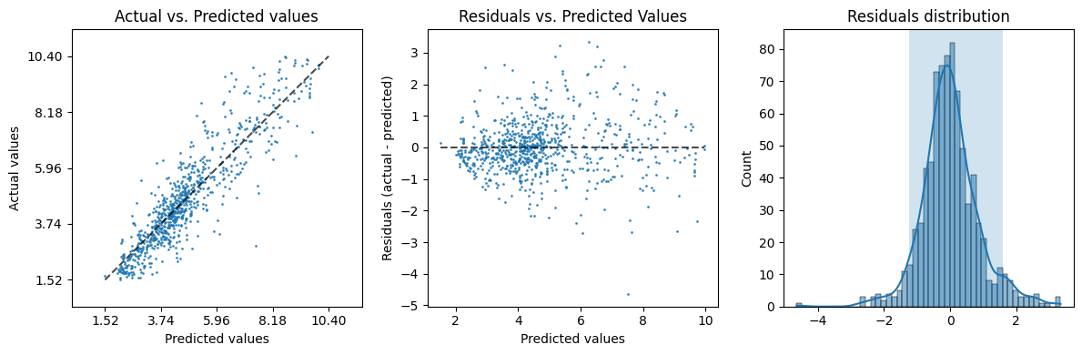
that depicts a some residuals (the difference between the true and the predicted values) analysis; in a more quantitative way we can inspect the metrics key, or the convenience version table:

print(evaluation['table'])

+-----------+---------+
| r2 mean   |  0.8028 |
| r2 std    |  0.0333 |
| rmse mean |  0.8617 |
| rmse std  |  0.0931 |
| q0        | -1.2509 |
| q1        |  1.5986 |
+-----------+---------+

Since the cross validation runs a model estimation per split (in this example, 5 times, that is the default value for the evaluation function), we get the mean and std (standard deviation) of two metrics of interest:

• the coefficient of determination (\(R^2\)) computed by r2_score(), and

• the root mean squared error (RMSE) computed by root_mean_squared_error().

Moreover, the evaluation returns the values of the empirical quantiles of the residual distribution (obtained using the mquantiles() function) \(q_0\) at 5% and \(q_1\) at 95%. The interval \([q_0, q_1]\) is the shaded box in the last of the three plots and represents the 90% of the residuals according to the cross validated prediction (obtained using the cross_val_predict() function).

A more robust boosting model

The HistGradientBoostingRegressor is a more recent implementation of the gradient boosting algorithm that is more efficient and can handle larger datasets, taking care of NaNs; we can use it with a simpler pipeline:

from sklearn.ensemble import HistGradientBoostingRegressor

regressor = HistGradientBoostingRegressor()
model =  make_pipeline(drop_all_nan_cols, regressor)
evaluation = evaluate_model(model, X, y)

result.append({'regressor': 'HistGradientBoosting'} | evaluation['metrics'])
evaluation['plot']

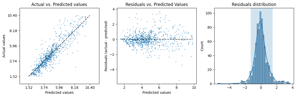
Quantitatively the results look promising:

print(evaluation['table'])

+-----------+---------+
| r2 mean   |  0.7982 |
| r2 std    |  0.0491 |
| rmse mean |  0.8692 |
| rmse std  |  0.1263 |
| q0        | -1.2855 |
| q1        |  1.4822 |
+-----------+---------+

A more precise tree model

We conclude this part with the ExtraTreesRegressor that seems to even even better performances.

from sklearn.ensemble import ExtraTreesRegressor

regressor = HistGradientBoostingRegressor()
model =  make_pipeline(drop_all_nan_cols, simple_imputer, standard_scaler, regressor)
evaluation = evaluate_model(model, X, y)

result.append({'regressor': 'ExtraTrees'} | evaluation['metrics'])
evaluation['plot']

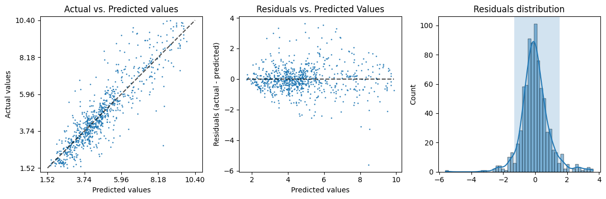
Quantitatively the results are even better:

print(evaluation['table'])

+-----------+---------+
| r2 mean   |  0.7959 |
| r2 std    |  0.0489 |
| rmse mean |  0.8745 |
| rmse std  |  0.1293 |
| q0        | -1.3052 |
| q1        |  1.5198 |
+-----------+---------+

Choose, train and save the model

We can put together the quantitative results to help us choose the best model:

from tabulate import tabulate

print(tabulate([r.values() for r in result], headers = result[0].keys(), tablefmt = 'outline', floatfmt = '.4f'))

+----------------------+-----------+----------+-------------+------------+---------+--------+
| regressor            |   r2 mean |   r2 std |   rmse mean |   rmse std |      q0 |     q1 |
+======================+===========+==========+=============+============+=========+========+
| GradientBoosting     |    0.8028 |   0.0333 |      0.8617 |     0.0931 | -1.2509 | 1.5986 |
| HistGradientBoosting |    0.7982 |   0.0491 |      0.8692 |     0.1263 | -1.2855 | 1.4822 |
| ExtraTrees           |    0.7959 |   0.0489 |      0.8745 |     0.1293 | -1.3052 | 1.5198 |
+----------------------+-----------+----------+-------------+------------+---------+--------+

Suppose we choose the last (ExtraTrees) model, we can then train it with all the data at our disposal

from jp2rt import save_model

model.fit(X, y)

Pipeline(steps=[('columntransformer',
                 ColumnTransformer(remainder='passthrough',
                                   transformers=[('drop_all_nan_cols', 'drop',
                                                  [216])])),
                ('simpleimputer', SimpleImputer()),
                ('standardscaler', StandardScaler()),
                ('histgradientboostingregressor',
                 HistGradientBoostingRegressor())])

In a Jupyter environment, please rerun this cell to show the HTML representation or trust the notebook.
On GitHub, the HTML representation is unable to render, please try loading this page with nbviewer.org.

Finally we can save the trained model using the save_model() function:

from jp2rt import save_model

save_model(model, 'extratrees')

315308

Use jp²rt

Even if performing the above tasks allows for a more detailed understanding of model estimation and can be personalized with further processing and analysis steps to improve the quality of the model, sometimes can be a tedious and error prone process, especially for beginners.

To facilitate the process we can use the simple_ensemble_model_estimate() function that takes as input the name of a regressor, valid names are returned by the list_ensemble_models() function:

from jp2rt import list_ensemble_models

list_ensemble_models()

['AdaBoost',
 'Bagging',
 'ExtraTrees',
 'GradientBoosting',
 'HistGradientBoosting',
 'RandomForest']

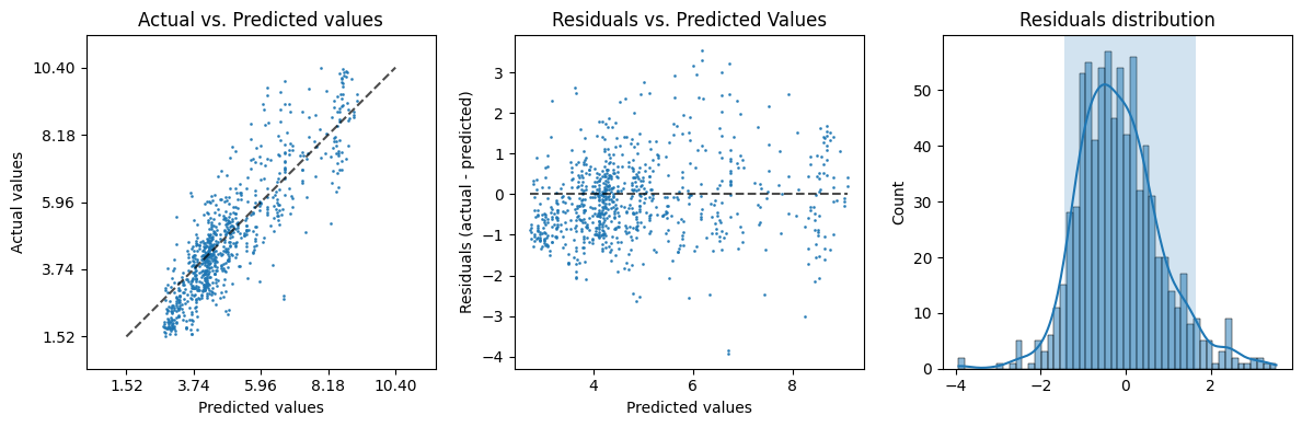
For example, we can see what we get using AdaBoost:

from jp2rt import simple_ensemble_model_estimate

model = simple_ensemble_model_estimate('AdaBoost', X, y)
evaluation = evaluate_model(model, X, y)
evaluation['plot']

The command line

To make things even easier, we can use the command line interface of jp²rt to list the available models:

$ jp2rt list-models

AdaBoost
Bagging
ExtraTrees
GradientBoosting
HistGradientBoosting
RandomForest

And to estimate (and evaluate) a model:

$ jp2rt estimate-model --evaluate Bagging docs/plasma+descriptors.tsv out

Read 799 molecules with 243 descriptor values each
Estimating model...

Model saved to /home/runner/work/jp2rt/jp2rt/docs/example/bagging.jp2rt (161647 bytes)...
Evaluating model...

+-----------+---------+
| r2 mean   |  0.7758 |
| r2 std    |  0.0286 |
| rmse mean |  0.9196 |
| rmse std  |  0.0824 |
| q0        | -1.4328 |
| q1        |  1.5489 |
+-----------+---------+

Evaluation plot saved to /home/runner/work/jp2rt/jp2rt/docs/example/bagging.png

that will create the bagging.jp2rt containing the saved model, and bagging.png the visual residual analysis.